OpenFOAM - Variation of Reynolds Number Across a Cylinder Section

Variation of Reynolds Number Across a Cylinder Section

Overview

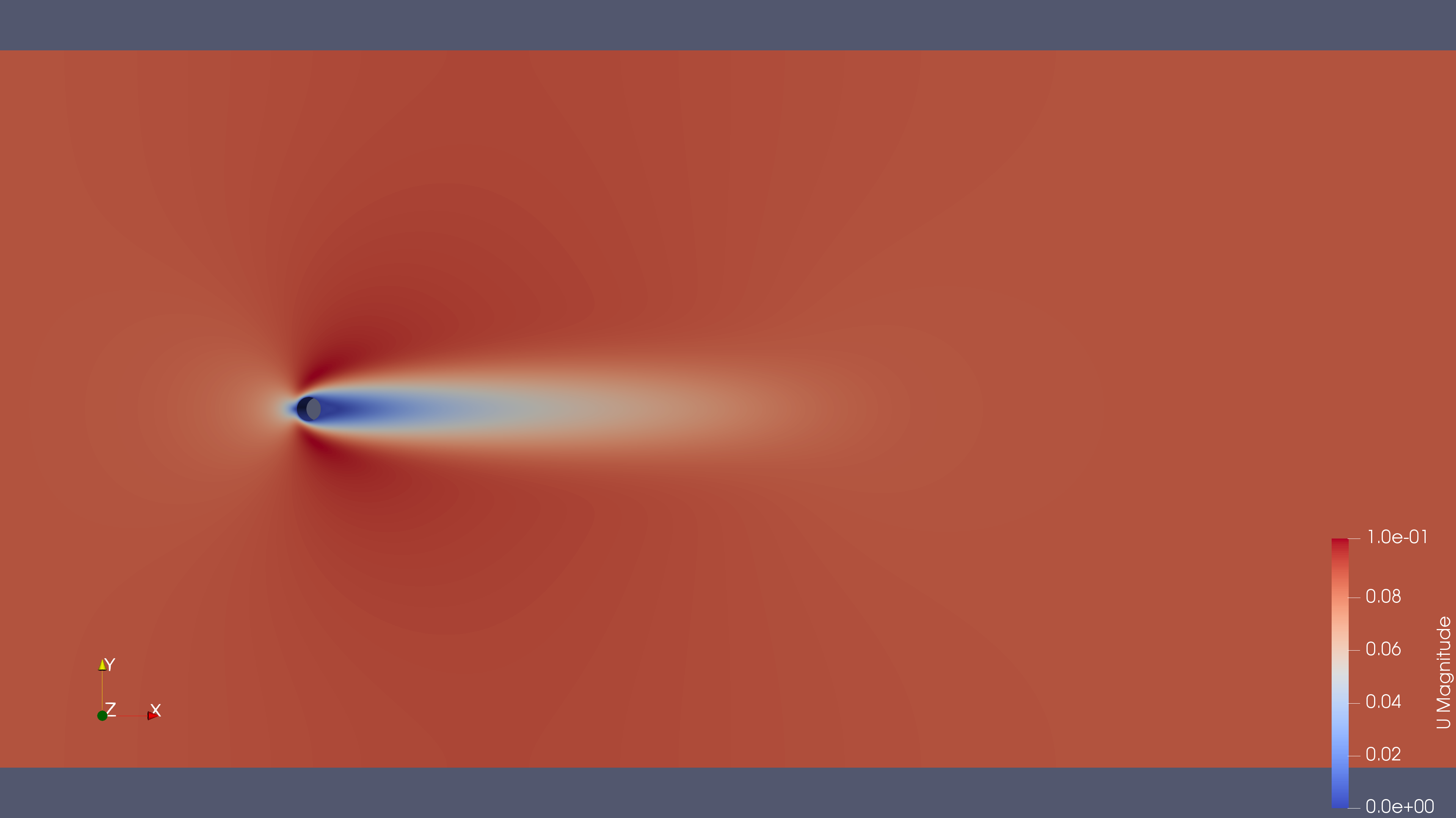
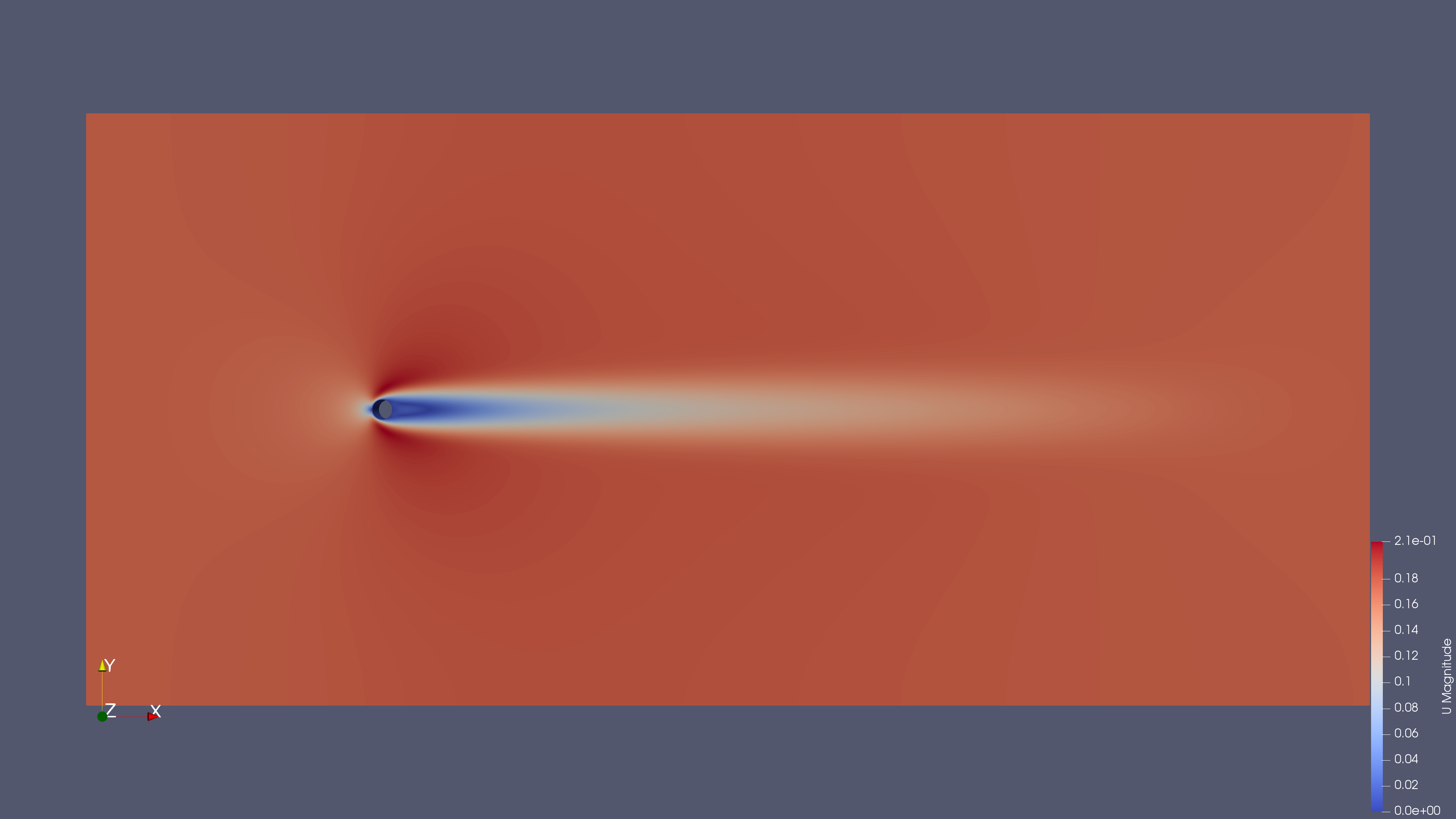
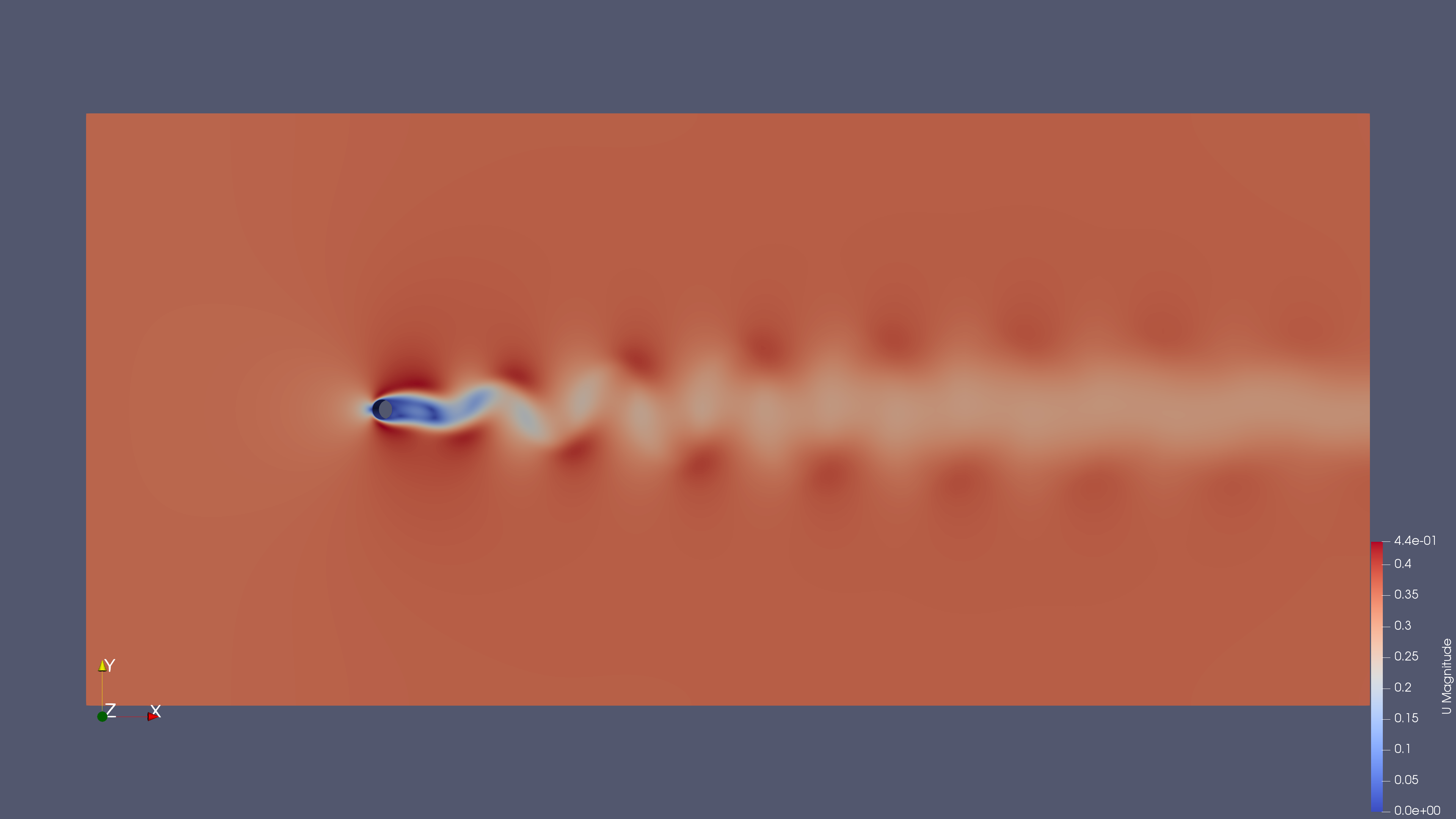
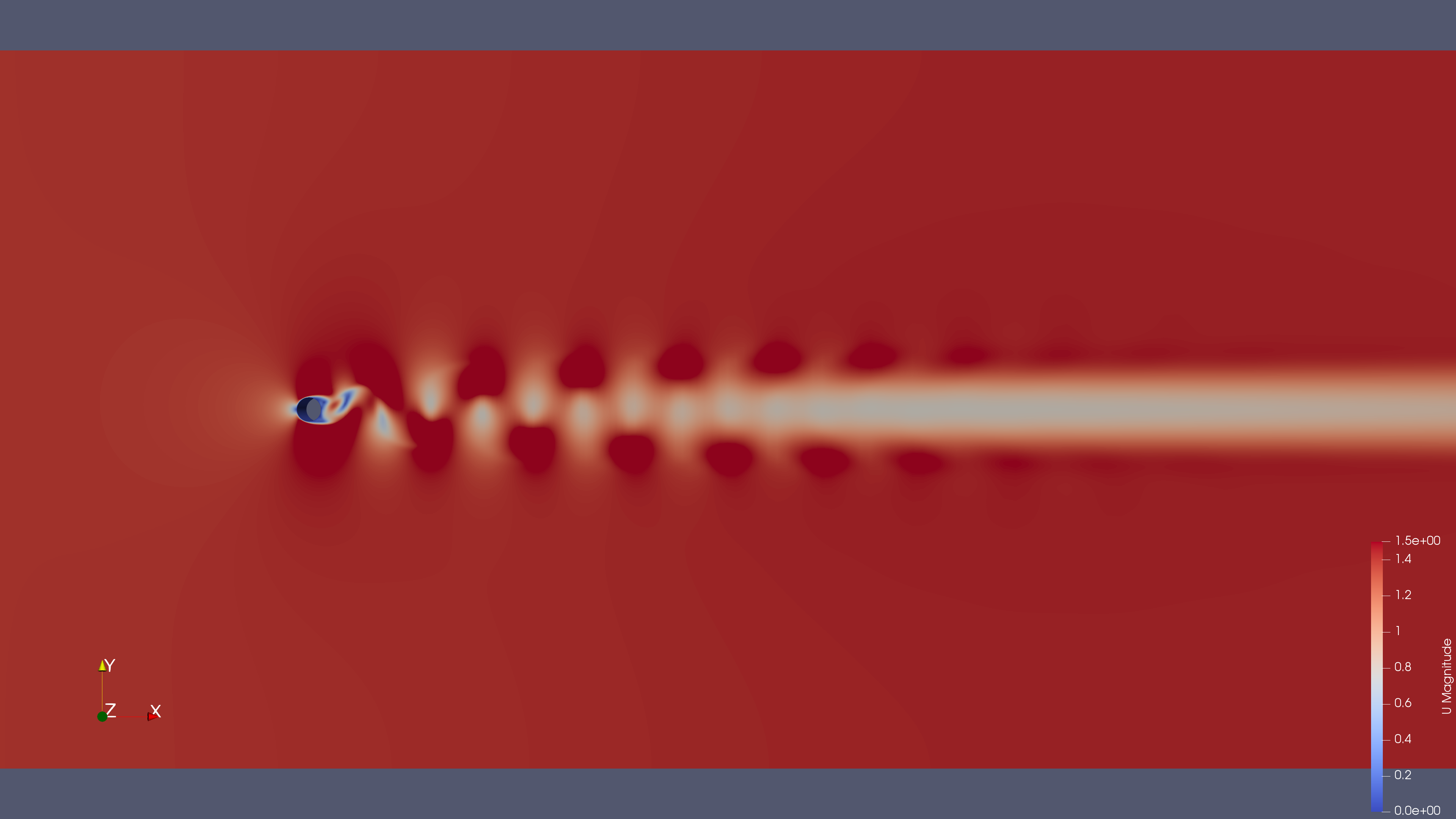
The following 4 videos and screenshots show flow over a cylinder of diameter 2mm for varying Reynolds numbers: 17.5, 35, 70 and 280. Transient simulations were set up for each of the simulations with the K-omega SST model deployed with appropriate values of K and omega assigned for each of the differing Reynolds numbers.

The 2D mesh used was very similar to that used in [1] and was created using ANSYS DesignModeller, resulting in a mesh of 78900 cells. FluentMeshtoFoam helped convert the exported ANSYS mesh into a mesh that OpenFOAM can use. Further work in this area could include refining the mesh and seeing the differences in the turbulence effects between the meshes. Finally, the simulations utilised 5 boundary conditions: inlet, outlet, walls (for the cylinder), symmetry (for the top and bottom) and frontAndBack.

Each simulation was set using the PISO algorithm such that it simulated up to 0.5 seconds of flow, giving plenty of time for the various turbulence effects to develop and propagate (if present). For the simulations with a Reynolds number of 17.5, 35 and 70, the deltaT used was 25 microseconds (as used in chapter 8.4 of Notes on Computational Fluid Dynamics: General Principles [2]). This resulted in the Courant number being well below 1 – the highest value from all 3 simulations was around 0.4. However, for the simulation with Reynolds number of 280 the deltaT had to be reduced to 20 microseconds, as early in the simulation the Courant number would spike and cause a crash. There were also issues with the Courant number when nCorrectors was set to 1, again spiking early in the simulation. This was set to 2, resolving those issues.

The simulation times varied between 30 and 50 minutes each, with the 280 Re simulation taking the longest time. DecomposePar was used to help speed up the simulations with the settings as follows:

numberOfSubdomains 14;

method hierarchical;

hierarchicalCoeffs {
    n (14 1 1);
    order xyz;
}

The hierarchical method was chosen for its good performance [3] and resulted in dramatically lower time when compared to the simple decomposition method (for this particular case). The following command was used to run the simulations: mpirun -np -14 -bind-to-core -bynode -use-hwthread-cpu pisoFoam -parallel. Early on in running these simulations, I noticed the workload was being split/shared across several threads instead of all the work being assigned to one thread, causing huge slow downs in my system. Therefore, I used -bind-to-core to help essentially ‘pin’ the workload to certain threads. The -use-hwthread-cpu allowed me to use the extra threads available on the processor (Ryzen 7 5800x) since it had only 8 physical cores but 16 total threads.

Below show videos of each of the 4 simulations and a screenshot of T = 0.5s. For equal comparisons between the videos, the range of U was set from 0 to 1.5m/s for all of them. The screenshots, however, were rescaled using the data just to see the turbulence effects more easily so the ranges of U will vary between them. The videos and screenshots show good agreement with data from [4], therefore giving some validation basis to the simulations. To properly validate these simulations, the lift/drag coefficients should be found from OpenFOAM and compared to experimental data, which is something to be done in the future.

Re = 17.5

Re = 35

Re = 70

Re = 280

References

[1] J. E. Matsson, An Introduction to ANSYS Fluent 2021, USA: SDC Publications, 2021

[2] C. J. Greenshields and H. G. Weller, Notes on Computational Fluid Dynamics: General Principles, Reading: CFD Direct, 2022

[3] S. Keough, Optimising the Parallelisation of OpenFOAM Simulations, Australian Government Maritime Division, 2014

[4] S. Taneda, Experimental Investigation of the Wakes behind Cylinders and Plates at Low Reynolds Numbers, The Physical Society of Japan, Vol 11, 1956