OpenFOAM - Drag Coefficient of Ahmed Body Across Multiple Reynolds Numbers
Overview
This section presents CFD simulations performed on an Ahmed body with a rear slant angle of 25 degrees. The objectives were to accurately model flow over an Ahmed body at various Reynolds numbers and to explore potential improvements for reducing the drag coefficients. Initially, the results of the mesh-independent study and preceding simulations are presented, followed by discussions regarding the processes/decisions made throughout the project, challenges faced while running the simulations, and so on.
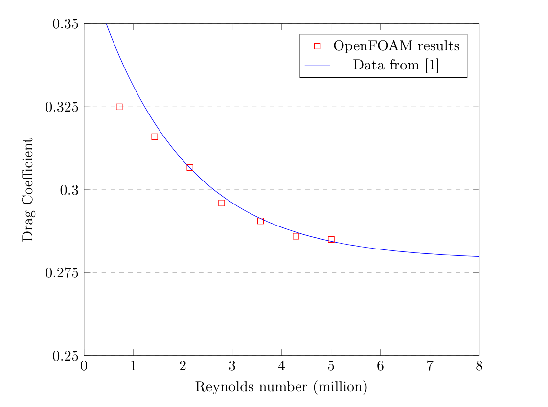
Work on the Ahmed body simulations began by estimating the approximate number of cells required, balancing both the accuracy of results and computation time. The mesh-independent study was carried out at a speed of 40m/s (Reynolds number of 2.784 million), with data from [1] indicating a target drag coefficient of around 0.299.
Originally, this section was meant to familiarize myself with snappyHexMesh to overcome limitations associated with meshing in ANSYS, which I had prior experience with (e.g., meshing with ANSYS in Windows, exporting, then shifting to Linux, given my separate drive with Linux). However, numerous challenges arose using snappyHexMesh, such as poor mesh quality in critical areas and extended meshing durations. Consequently, cfMesh was employed for this study. A key benefit of cfMesh is its requirement of just a single file to initiate the meshing process: meshDict. Moreover, cfMesh generates meshes more swiftly than snappyHexMesh—a boon since multiple meshes were needed. Careful consideration ensured a suitable distribution of cells (i.e., a higher cell concentration in critical areas and fewer at external boundaries) to accurately report the drag coefficient.
After mesh generation and validation via OpenFOAM’s checkMesh command, the simulations utilized the k-omega SST model (with k and omega based on values from [2]), the SIMPLE algorithm, and ran for 500 iterations with a time step of 1 second. Designating 500 iterations let the drag coefficient change to an extent where the suitability of a specific cell count could be assessed.
The mesh independence study results are displayed in the subsequent figures, detailing both the projected drag coefficient and the average reported y+. Achieving a mesh with a cell count between 4 and 6 million of acceptable quality proved challenging, thus only three meshes were evaluated in the study.
The percentage discrepancy between the theoretical and predicted drag coefficients for the mesh of ~6.5 million cells stood at 1.01%. For ~3.1 million cells, it was 3.34%, and for ~2.5 million cells, it was 13.71%. The ~6.5 million cell mesh required 1.605 hours for 500 iterations, while the ~3.1 million and ~2.5 million cell meshes took 0.76 and 0.64 hours respectively. At a glance, the ~3.1 million cell mesh might seem optimal in terms of precision and time. However, the average y+ for the ~3.1 million cell mesh was approximately 14.22 on the Ahmed body, which isn’t satisfactory for the k-omega SST model close to the Ahmed body walls. Hence, the ~6.5 million cell mesh was chosen for subsequent simulations. Additionally, both the ~2.5 and ~3.1 million cell meshes struggled to accurately predict the recirculation zone at the body’s rear, as demonstrated in the following figures.
Mesh Independence Study 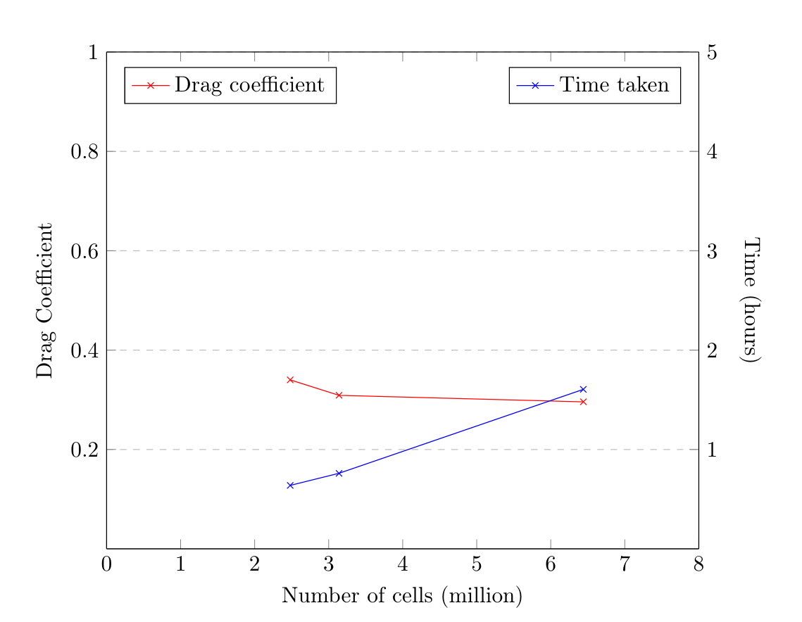
Y+ Graph 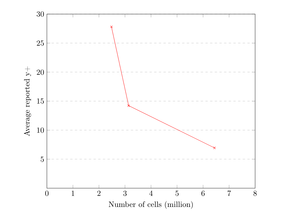
Incorrect recirculation zone 
Correct recirculation zone 
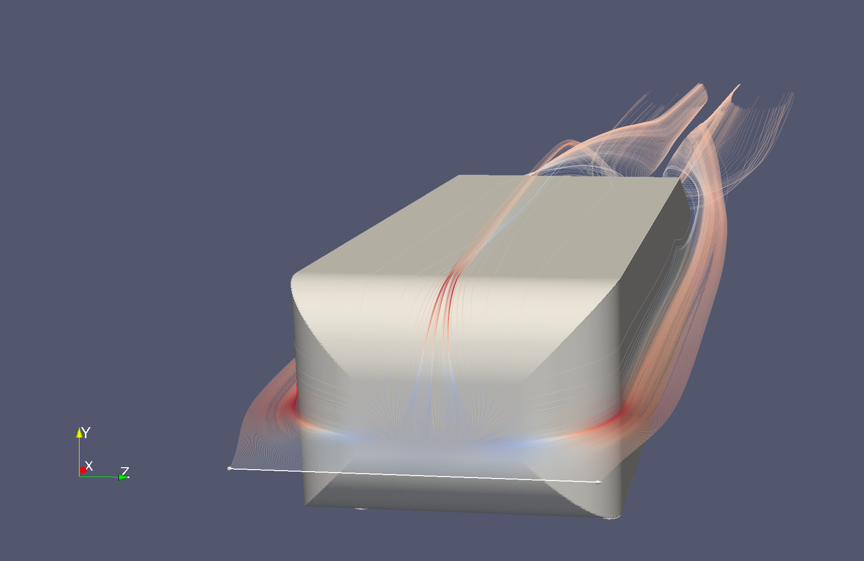
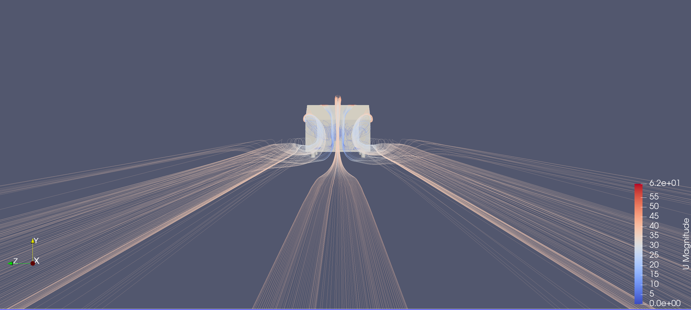
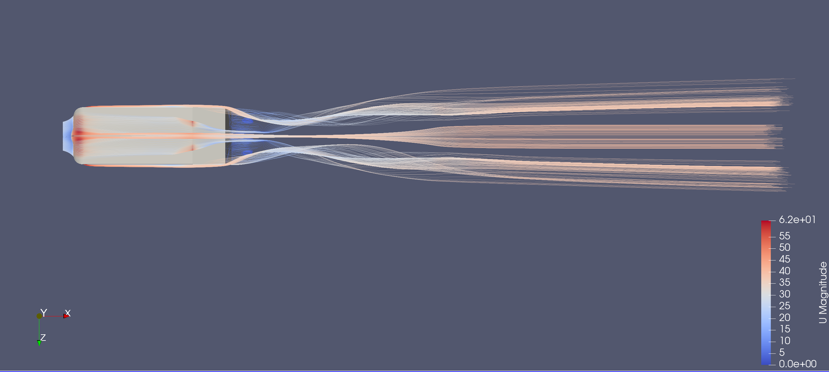
Predicted Vortex Sheet & Drag Coefficient at Different Reynolds Numbers
The following images show the predicted vortex structures and results for the drag coefficient at different Reynolds numbers.
Reducing The Drag Coefficient
Investigations to reduce the drag coefficient included simple modifications to the Ahmed body, including rounding regions on the top and the rear of the model. In total, 5 models were produced, named from A to E, with the following modifications:
Base Model:
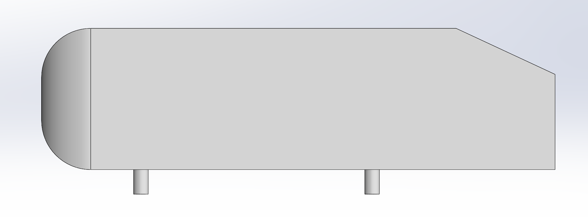
Model A - a 50mm fillet where the 25 degree slant begins 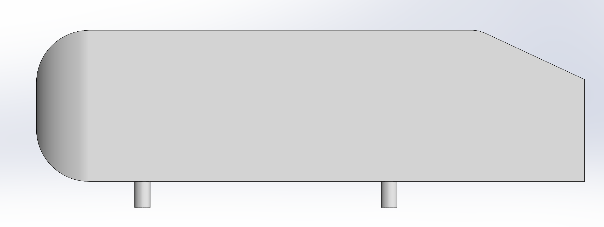
Model B - a 50mm fillet where the 25 degree slant ends 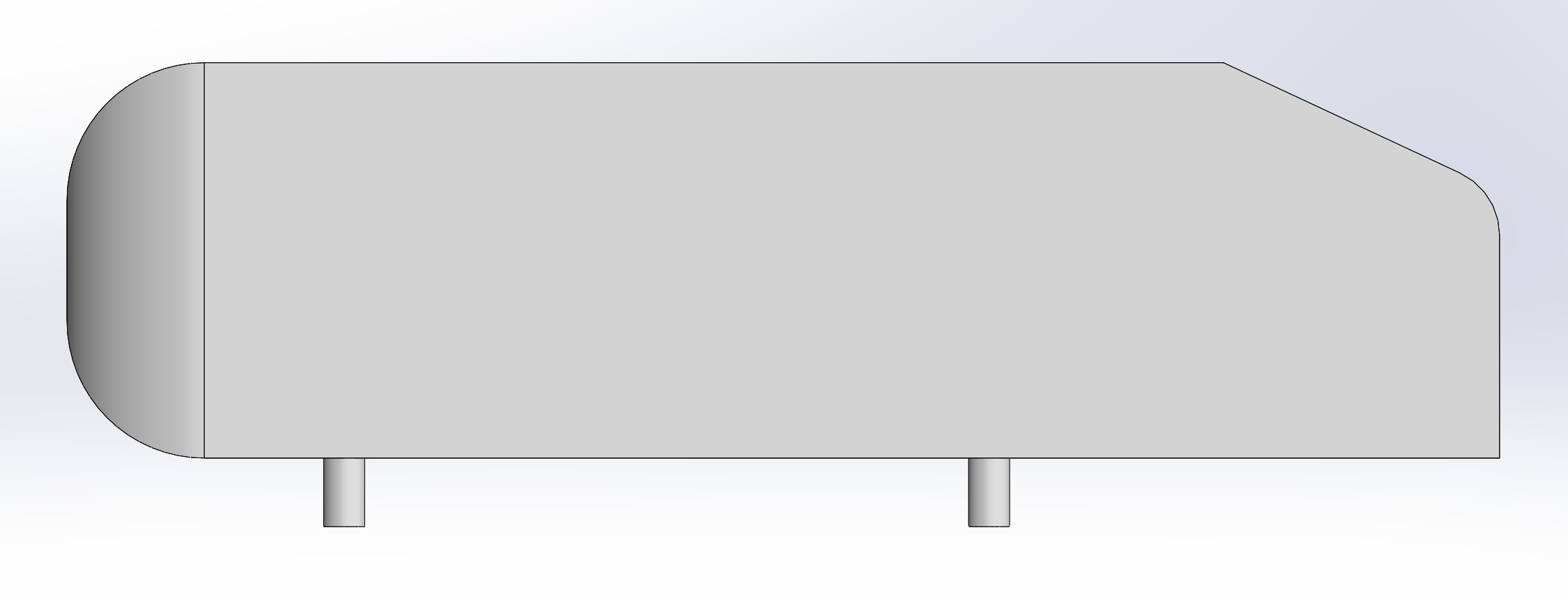
Model C - a 50mm fillet on the underside at the rear of the body 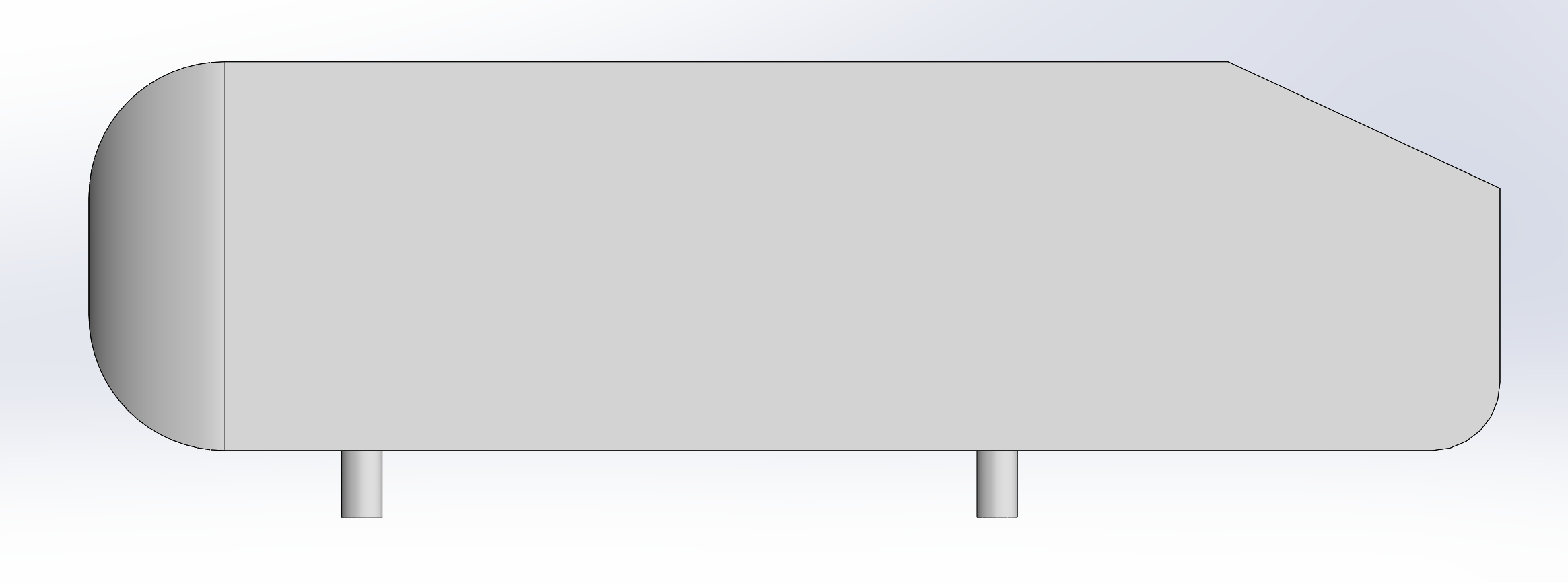
Model D - 50mm fillets where the 25 degree slant begins and on the underside at the rear of the body 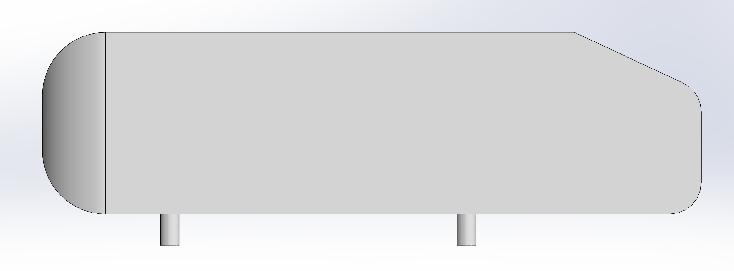
Model E - 50mm fillets in all of the previous locations 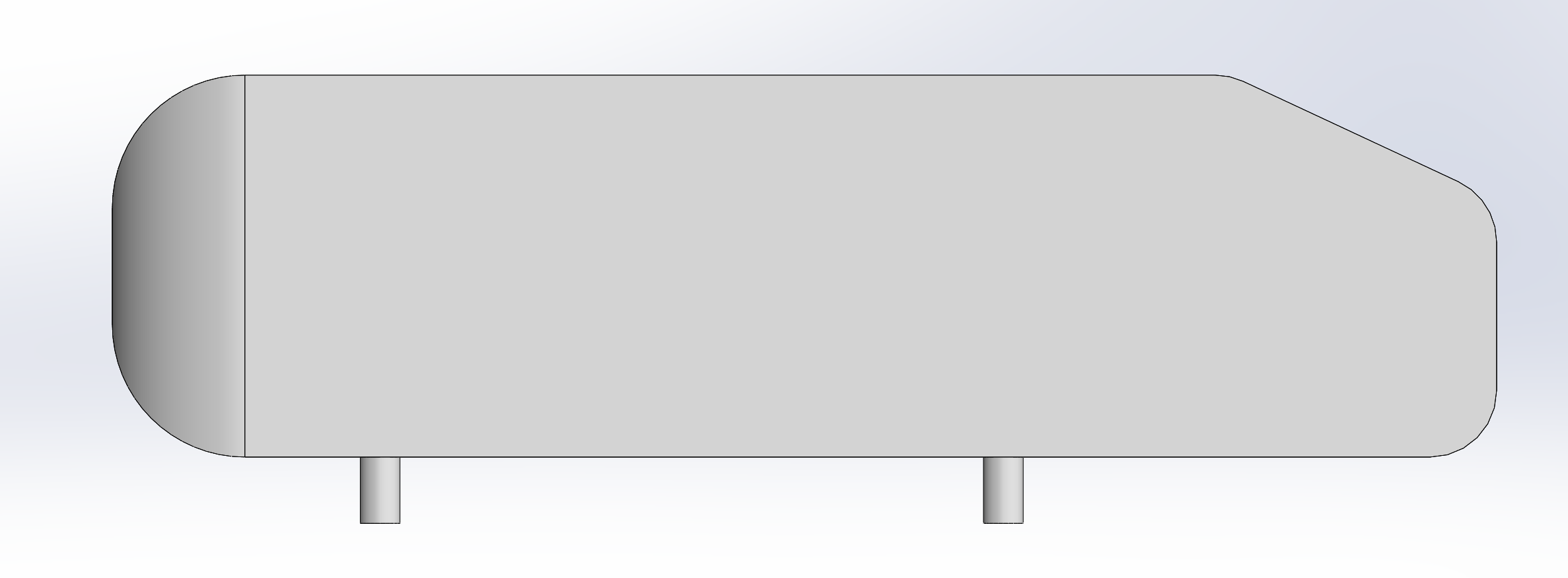
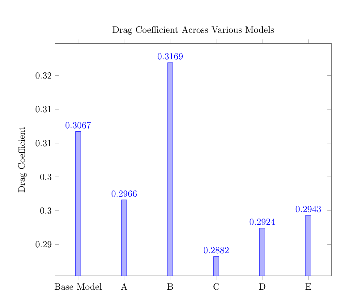
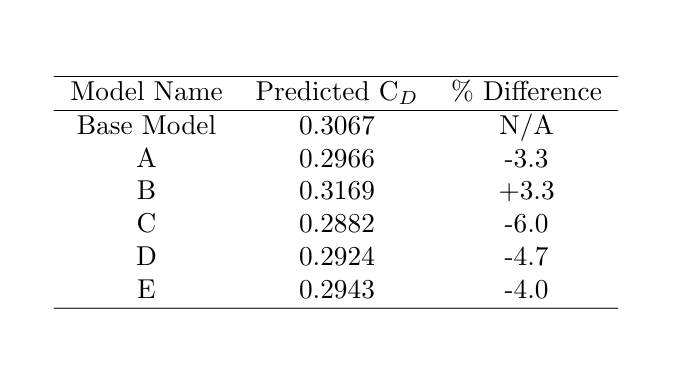
Each simulation was ran at with a Reynolds number of 2.145 million and used the same mesh settings as the ideal mesh in the mesh independence study, meaning the results should have a good degree of credibility. Ideally, each simulation could be verified with wind tunnel experiments but unfortunately I don’t have access to one. Below, you’ll find a bar chart summarising the simulation results, flow screenshots across the body and a brief summary of the finding from each model. From hereon, the unmodified Ahmed body will be referred to as ‘base model’.
Model A:
- Model A exhibits a 3.3% reduction in drag coefficient compared to the base model.
- The sharp, convex turn on the base model disrupts airflow, causing the air to detach over the rear slant.
- A side profile view clearly illustrates this difference (see Figures 1 and 2).
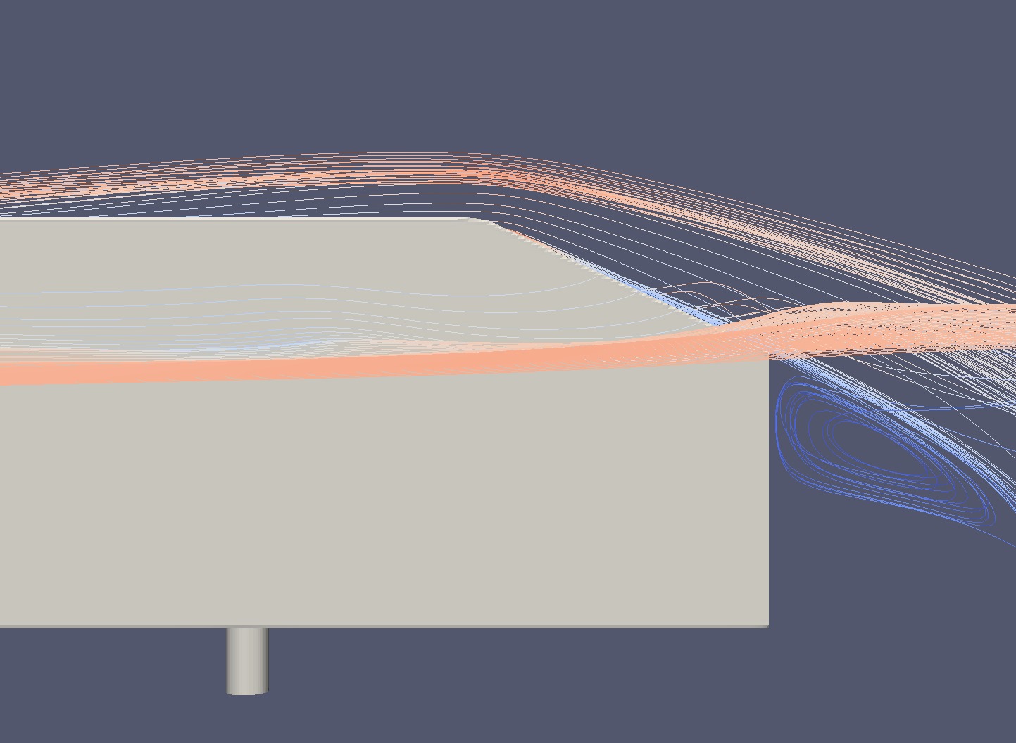
Figure 1: With rounded top
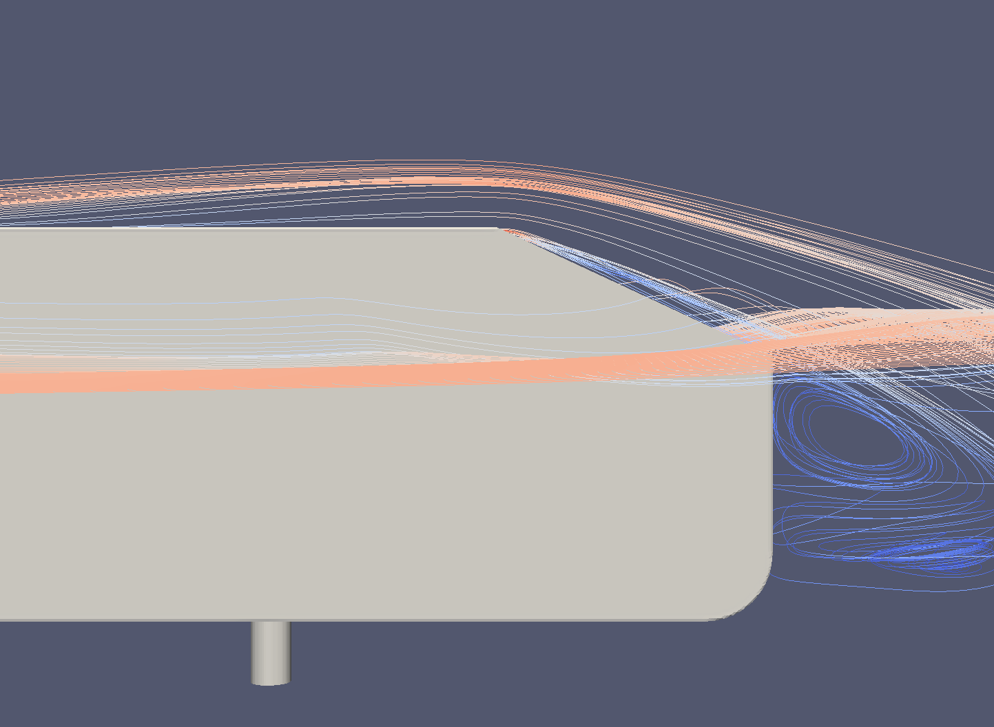
Figure 2: With sharp top
Model B:
- Model B is predicted to have a 3.3% higher drag coefficient compared to the base model.
- Models with a similar feature to Model B cause side vortex structures to wrap around more (Figure 3) prominently over itself and have a wider vortex sheet.
- A front/top view reveals this effect (Figure 4 and 5)
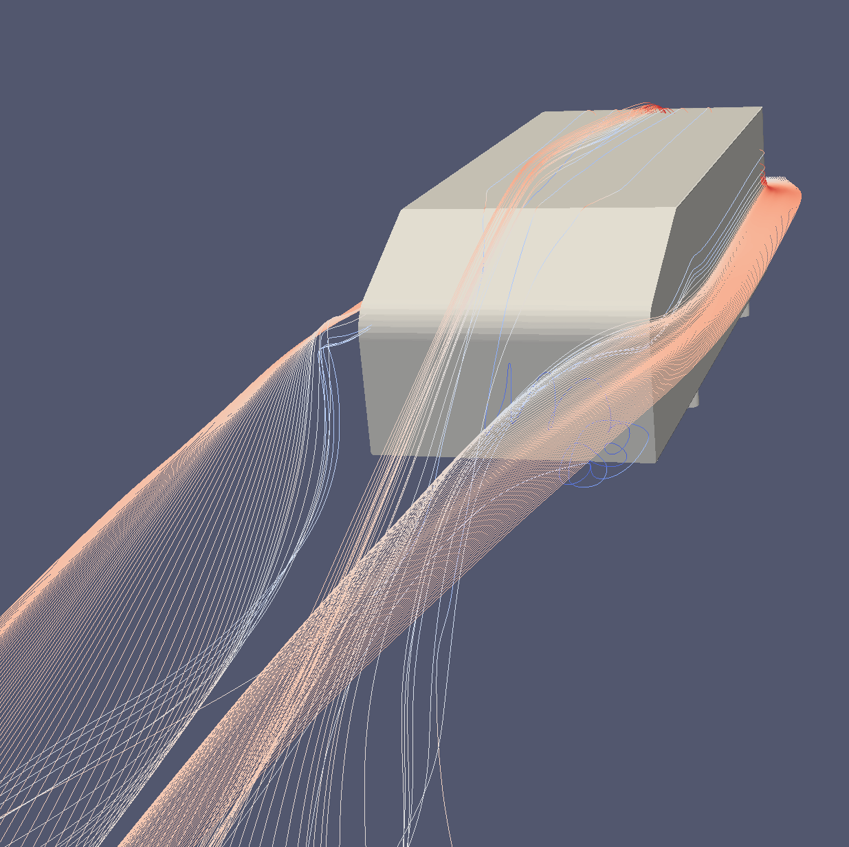
Figure 3: Vortex sheet wrapping more around itself
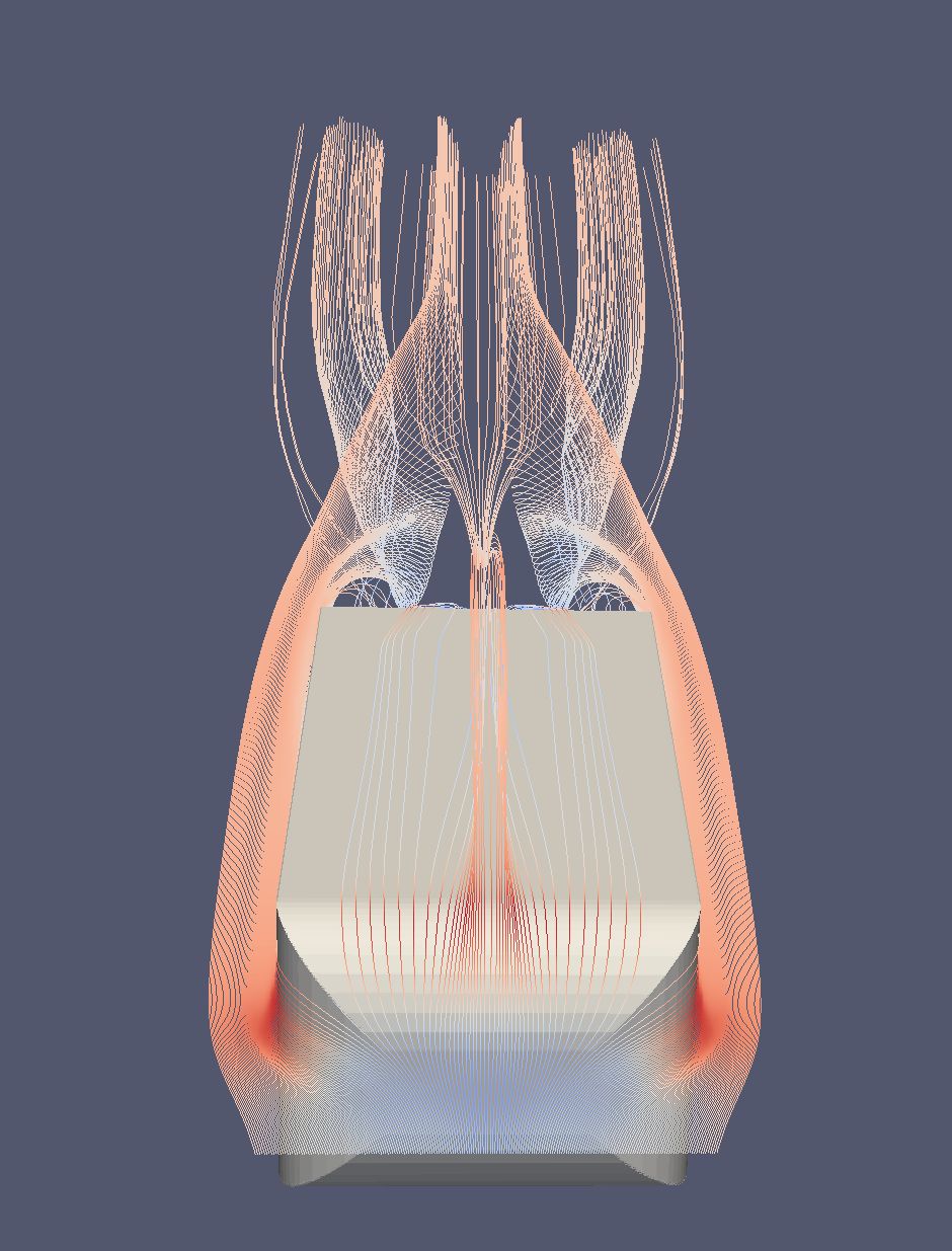
Figure 4: Wider vortex sheet with rounded top-rear
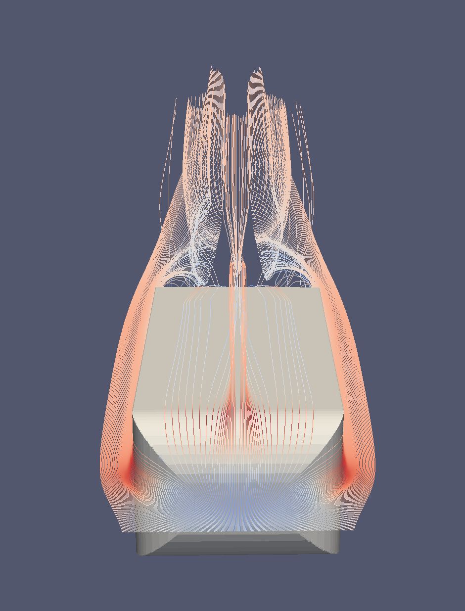
Figure 5: Narrower vortex sheet without rounded top-rear
Model C:
- Model C is expected to have a 6.0% lower drag coefficient compared to the base model.
- The rounded bottom rear allows air to flow more smoothly, especially after the rear of the body (Figure 6 and 7)
- Using an isometric view, the vortex structures from the underside of the model are seen to follow a straighter path (Figure 8 and 9)
- The rounded bottom rear forces vortex structures on the edge of the body to meet with the side vortex structures.

Figure 6: With rounded bottom-rear

Figure 7: Without rounded bottom-rear
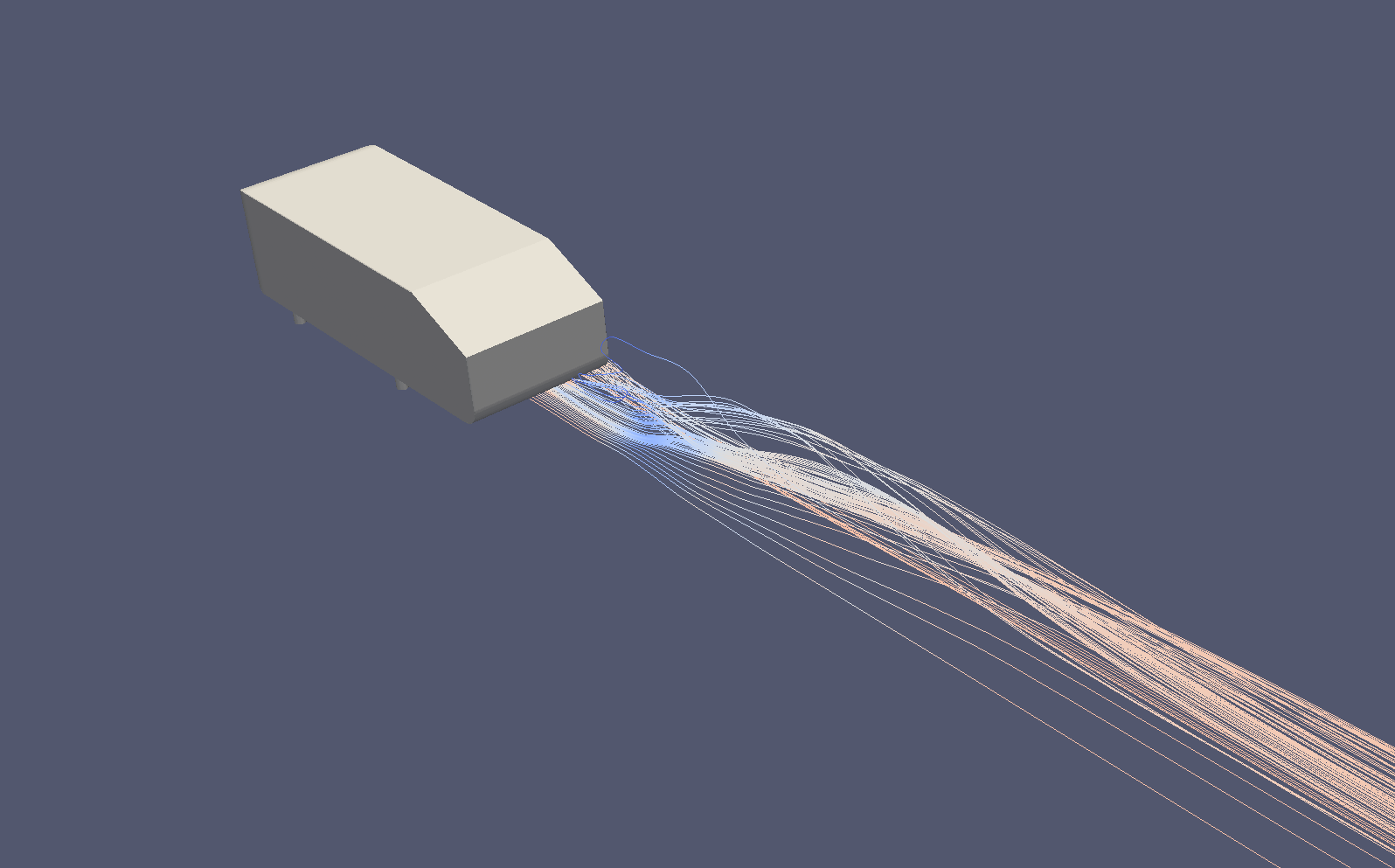
Figure 8: With rounded bottom-rear
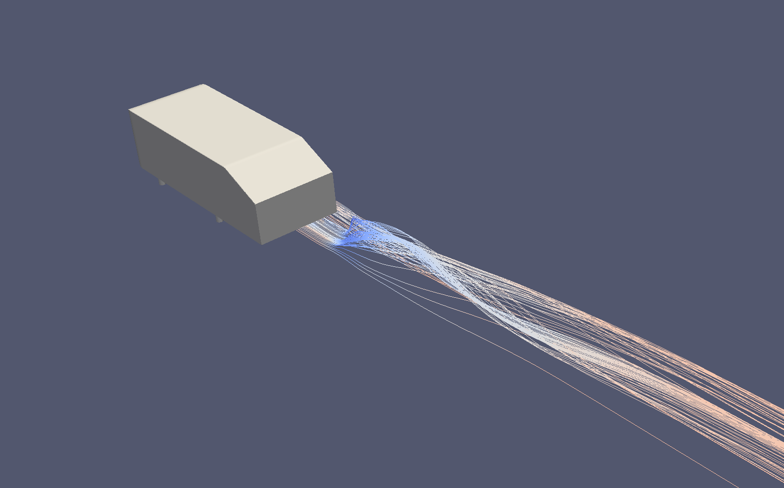
Figure 9: Without rounded bottom-rear
Model D & E:
- Models D and E share features with Models B and C, respectively.
- It’s expected that they would have lower drag coefficients than Model B (due to the rounded bottom rear) and higher than Model C (due to the rounded top rear), as confirmed by the bar chart.
- Notably, Model E, with three regions of curvature, has a higher predicted drag coefficient than Model D, suggesting that the features present in Models B and D don’t work well together.
Results:
Results from the drag coefficient reduction modifications
Issues During Early Simulations
Early on in the mesh independent study, the following settings for the divSchemes in fvSchemes were used for initial testing:
divSchemes
{
    default none;
    div(phi,U) Gauss upwind;
    div(phi,k) Gauss upwind;
    div(phi,omega) Gauss upwind;
    div((nuEff*dev2(T(grad(U))))) Gauss linear;
}
These worked fine (as expected, seeing as they are first order schemes) and when tests were run with second order schemes, issues started to arise. The first set of second order schemes to be used were as follows:
divSchemes
{
    default none;
    div(phi,U) Gauss linearUpwind grad(U);
    div(phi,k) Gauss linearUpwind grad(k);
    div(phi,omega) Gauss linearUpwind grad(omega);
    div((nuEff*dev2(T(grad(U))))) Gauss linear;
}
After around 200 iterations, the simulation would crash and report floating point errors. Using the above settings led to a value for bounding k and bounding omega to be reported during solving, and when the simulation crashed, these values would be extremely large (above 1e150). A lot of time was spent trying to remedy this issue, such as changing the mesh and ensuring initial value of k and omega were set correctly. Despite the first order schemes for div(phi,k) and div(phi,omega) resulting in stable and accurate (when looking at the drag coefficient) solutions, they could not be used for the final simulations as they caused incorrect predictions of flow on the slope of the rear of the Ahmed body. After some research (and a lot of headaches), the following settings led to: a) an acceptable difference between the theoretical and predicted drag coefficients and b) correct predictions of flow over the Ahmed body:
divSchemes
{
    default none;
    div(phi,U) bounded Gauss limitedLinear 1.0;
    div(phi,k) bounded Gauss upwind;
    div(phi,omega) bounded Gauss upwind;
    div(phi,epsilon) bounded Gauss upwind;
    div((nuEff*dev2(T(grad(U))))) Gauss linear;
}
With the issue of the crashing and inaccuracies resolved, the resulting fvScheme files looked like so (Bearing in mind the majority of meshes used had a maxOrthogonality less than 60):
FoamFile
{
    format ascii;
    class dictionary;
    object fvSchemes;
}
FoamFile
{
    format ascii;
    class dictionary;
    object fvSchemes;
}

ddtSchemes
{
    default steadyState;
}

gradSchemes
{
    default cellMDLimited Gauss linear 0.0; be oscillatory on tetrahedral meshes
    grad(U) cellLimited Gauss linear 0.5;
}

divSchemes
{
    default none;
    div(phi,U) bounded Gauss limitedLinear 1.0;
    div(phi,k) bounded Gauss upwind;
    div(phi,omega) bounded Gauss upwind;
    div(phi,epsilon) bounded Gauss upwind;
    div((nuEff*dev2(T(grad(U))))) Gauss linear;
}

laplacianSchemes
{
    default Gauss linear limited 0.75;
}

interpolationSchemes
{
    default linear;
}

snGradSchemes
{
    default limited 0.75;
}

wallDist
{
    method meshWave;
}
Whilst cfMesh was quite pleasurable to use, it did have some quirks that casued a few headaches. The following excerpt from the meshDict was used to determine the meshes throughout MIS:
surfaceFile "ahmedbodywithbox.fms";
maxCellSize X;
keepCellsIntersectingBoundary 0;

objectRefinements
{
    mainBox
    {
        type box;
        cellSize X; //[m]
        centre (1.125 0 0); //[m]
        lengthX 2.5; //[m]
        lengthY 1; //[m]
        lengthZ 1.5; //[m]
    }
}

localRefinement
{
    solid
    {
        cellSize X;
        refinementThickness X;//[m]
    }
}
Originally, since the height of the domain was two metres, it was decided to have the maxCellSize as numbers that would go into two (e.g. 0.1, 0.2, 0.4, 0.5 and so on to ensure even cells at the boundaries). Setting the maxCellSize as these often ramped up the cell count (going above 10 million, and even 20 million in some cases). If the maxCellSize was set to something different, such as 0.15, 0.3, 0.45, then the cell counts would be much lower and within an acceptable limit (thereby drastically reducing simulation time). Setting the boundary layers above 10 layers also caused extremely poor quality meshes, so 5 layers were used throughout all of the meshes.
References
[1] Meile et al., Experiments and numerical simulations on the aerodynamics of the Ahmed body, CFD Letters 3(1), 2011
[2] “Flow around the Ahmed body - Validation Case - SimFlow CFD,” help.sim-flow.com. https://help.sim-flow.com/validation/ahmed-body